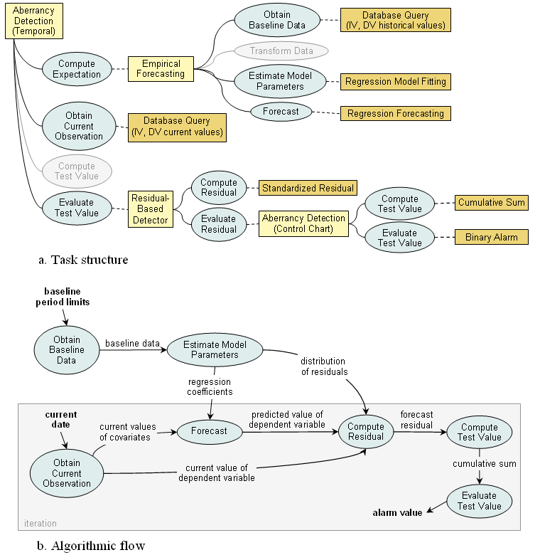
Representation of a two-stage detection algorithm combining regression modeling and control chart

The data forecasts for this algorithm are generated based on previous observations. So Empirical Forecasting TDM is used again to perform Compute Expectation task. Typical of any regression-based approach, this algorithm requires a considerable amount of historical data for model fitting. All the data is provided at once by the method performing Obtain Baseline Data task, and it usually includes multiple time series (at least one independent and one dependent variable). The data are then passed to a Regression Model Fitting method to estimate regression parameters in Estimate Model Parameters task. The Forecast task is performed by a Regression Forecasting method, which uses the parameterized regression model and current values of the covariates to compute the expected value.

The Obtain Current Observation task is similar to the previous examples in the sense that only a single observation is retrieved at a time. However, the observation includes current values of all covariates (as specified by the model) for a given test period in addition to the value of the dependent variable. As in the Holt-Winters approach, the current observation (dependent variable) is used directly as a test statistic, thus the Compute Test Value task is skipped.

The Evaluate Test Value task is decomposed further into two subtasks: first the standardized forecast residual is computed by the Compute Residual task, and then the value of this residual is passed to the second stage of aberrancy detection. The Evaluate Residual task here is performed by an Aberrancy Detection task-decomposition method, in particular a CUSUM control chart. This method is represented using the same general task structure for the aberrancy detection algorithms, though largely simplified due to omitted subtasks. In particular, the Obtain Baseline Data and Estimate Model Parameters tasks will be skipped, since the distribution of residuals is known from fitting the regression model; no query is needed to Obtain Current Observation, as the previously computed value of residual is readily available; and as in all control charts, the Compute Expected Value task can be skipped. So essentially, the algorithm is reduced to just two tasks: Compute Test Value task using a Cumulative Sum method and Evaluate Test Value task using a Binary Alarm method (the omitted tasks are not displayed in the figure).

Figure b shows data flow and iteration control for this algorithm. The regression model fitting step and preceding query for baseline data are not repeated at each execution step, but are performed only once. These tasks are thus outside iteration container.

← Back to Models